The 10 Most Important Excel Functions (With Examples)

The Excel functions most people need are SUM to add, AVERAGE for the mean, COUNT and COUNTA to count, MAX and MIN for the highest and lowest values, IF for conditions, COUNTIF and SUMIF to count and add with a condition, VLOOKUP and XLOOKUP to look things up, and IFERROR to handle errors. Master these ten and you've covered most everyday spreadsheet work.

In short: every function starts with =, then the function name, then its arguments in brackets. Learn the basic maths functions first, then conditions, then lookups.

Before you start: how to write a function in Excel

All the examples use one simple sales table: column A has employee names, column B has the city, column C has sales, and the data runs from row 2 to row 11.

The basic rules:

• Start every formula with =.
• As you type the first letters of a function, such as =SU, Excel shows a list of suggestions. Pick the function and press Tab to complete it, and a tooltip under the cell shows the order of its arguments.
• A range like C2:C11 means every cell from C2 down to C11.
• Put text inside double quotes, like "London".
• After typing a formula, drag the small square in the corner of the cell to copy it down to other rows.
• To keep a reference fixed when you copy a formula, write it as $F$1, or press F4 while typing it.

=C2*$F$1

Here C2 becomes C3, then C4 as you drag the formula down, while $F$1 stays put. That's handy when a single cell holds something like a commission rate.

The basic maths functions

1. SUM: add numbers

=SUM(C2:C11)

Adds up all the sales. Quick tip: select the cell under a column of numbers and press Alt + = and Excel writes the SUM for you.

2. AVERAGE: the mean

=AVERAGE(C2:C11)

Works out average sales. Watch out: empty cells are ignored, but cells containing zero are included.

3. COUNT and COUNTA: counting

=COUNT(C2:C11)
=COUNTA(A2:A11)

COUNT only counts cells that contain numbers. COUNTA counts every non-empty cell, text or number. Use COUNTA on the names column to find how many employees you have.

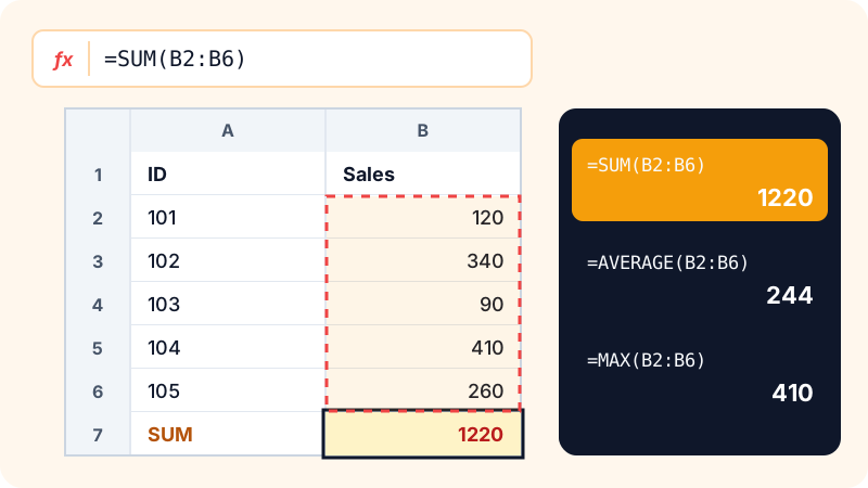
4. MAX and MIN: highest and lowest

=MAX(C2:C11)
=MIN(C2:C11)

5. IF: let Excel make the decision

IF tests a condition and returns one result if it's true and another if it's false:

=IF(C2>=5000, "Excellent", "Needs follow-up")

You can nest one IF inside another to handle more cases:

=IF(C2>=5000, "Excellent", IF(C2>=3000, "Good", "Low"))

If you have Microsoft 365 or Excel 2019 or later, the IFS function is easier to read when you have several conditions:

=IFS(C2>=5000, "Excellent", C2>=3000, "Good", TRUE, "Low")

Counting and adding with conditions

6. COUNTIF and COUNTIFS

=COUNTIF(B2:B11, "London")
=COUNTIF(C2:C11, ">5000")
=COUNTIFS(B2:B11, "London", C2:C11, ">5000")

The first counts employees in London, the second counts everyone with sales above 5,000, and the third needs both conditions to be true.

Instead of typing the condition into the formula, you can put it in its own cell and point to it, so you can change the condition without editing the formula. Note that a comparison sign goes in quotes and is joined to the cell with &:

=COUNTIF(B2:B11, E1)
=COUNTIF(C2:C11, ">"&E2)

Type the city in E1 and the minimum sales figure in E2, and the result updates whenever you change either one.

7. SUMIF and SUMIFS

=SUMIF(B2:B11, "London", C2:C11)
=SUMIFS(C2:C11, B2:B11, "London", C2:C11, ">1000")

Note the different argument order: in SUMIF the range to add comes last, while in SUMIFS it comes first, followed by the condition pairs. This trips up almost everyone at least once.

Looking up data: VLOOKUP and XLOOKUP

8. VLOOKUP

=VLOOKUP("Sara", A2:C11, 3, FALSE)

Looks for "Sara" in the first column of the range and returns the value from the third column of that range (sales). Always put FALSE at the end for an exact match. The default is an approximate match, which can quietly return the wrong result.

9. XLOOKUP

=XLOOKUP("Sara", A2:A11, C2:C11, "Not found")

Simpler and more flexible: you choose the lookup column and the result column separately, exact match is the default, and you can say what to show when nothing is found.

	VLOOKUP	XLOOKUP
Can look to the left	No	Yes
Default match	Approximate	Exact
Breaks when you insert columns	Yes, the column number is fixed	No
Available in	All versions	Microsoft 365, Excel 2021 and later

10. IFERROR: hide error messages

=IFERROR(XLOOKUP("Sara", A2:A11, C2:C11), "Not found")
=IFERROR(C2/D2, 0)

Returns the result if there's no error, and your fallback value if there is. Use it with care: it hides every kind of error, including ones you actually need to see and fix.

Small functions worth knowing

=TRIM(A2)
=ROUND(C2*0.15, 2)
=A2 & " - " & B2

• TRIM removes extra spaces from text. It's a lifesaver with data copied from websites or other systems.
• ROUND rounds a number to the number of decimal places you choose.
• The & operator joins text together, giving you something like "Sara - London".

Stuck on a complicated formula? Describe what you want to an AI tool like ChatGPT, ask it for the formula, then test the result on your own data. Our guide on how to write good prompts shows how to ask clearly, and if you're new to these tools, start with the ChatGPT beginner's guide.

Common errors and what they mean

Error	What it means	Fix
#N/A	The value you looked up wasn't found	Check spelling and spaces, try TRIM
#DIV/0!	Division by zero or by an empty cell	Check the divisor or wrap it in IFERROR
#VALUE!	Wrong data type, such as text instead of a number	Make sure the cells really contain numbers
#NAME?	Misspelled function name or text without quotes	Check the spelling and the quotes
#####	The column is too narrow for the value	Widen the column

To work even faster, learn the Windows keyboard shortcuts worth knowing. Many of them, like Ctrl + C and Ctrl + Z, work in Excel too.